Tuesday, July 29, 2014

It’s all about the variance: science and life at N > 2

Variation is the grist for, and the flour from, the evolutionary mill. Without variation, no evolution occurs. With variation, evolution can generate even more variation by causing organisms in different environments to evolve different traits. We all know this, and we proceed accordingly in our research; but perhaps we too often take it for granted. Only sometimes are we smacked in the face by variation in such a way that it makes us pause and re-evaluate the way we view the world. Well, variation smacked me upside the head a few weeks ago during a trip into the field. In so doing, it made me reflect on how we estimate and interpret variance – and how this flavors the way we view our research and our daily experiences.

Threespine stickleback (Gasterosteus aculeatus)
Threespine stickleback could be the world’s most variable vertebrate. In some populations, average size at maturity is less than 30 mm – in others it is greater than 85 mm. In some populations, the pelvis is a huge structure – in others it is completely lacking. In some populations, the side of the fish is almost completely covered with bony plates – in others plates are entirely absent.  In some populations, mature males are almost entirely black – in others they have massive amounts of red – and in others black and red can be minimal. In some populations, the head is huge and the mouth massive – in others they are very small. In some populations, mean egg size (dry mass) is less than 0.047 mg – in others it is greater than 0.089 mg. This is just a small set of examples: stickleback, even just in freshwater, vary dramatically both within and among populations in almost any trait one cares to measure. This is why they are such a spectacular model system for studying adaptation.

A representation of stickleback diversity. The marine ancestor is surrounded by various freshwater forms.
Tom Reimchen, a professor at the University of Victoria, has long maintained that variation in stickleback on Haida Gwaii, a modest-sized archipelago off the coast of northern British Columbia, Canada, are as variable as are stickleback across the rest of their massive range in the northern hemisphere. Ever the skeptic, I have – when reviewing or editing Tom’s papers – pointed out that this assertion isn’t strictly true as (slightly) smaller stickleback are found in North Uist, Scotland. I am sure my nit was annoying to Tom as it was just a technicality and it required him inserting some rather pointless qualifiers into a few of his papers.


Several weeks ago, I had the opportunity to visit Tom in the field to see Haida Gwaii stickleback for myself. The first lake we visited was Drizzle, where Tom lived for 15 years and worked for 40. Drizzle is a modest-sized (112 ha) and heavily-stained (tannic, the color of very strong tea) lake with large and dark stickleback. A highlight here (besides camping and having a breakfast of bannock beside the lake) was walking the shoreline on Tom’s annual survey of loon-induced stickleback mortality. Several species of loon, particularly common and red-throated loons, congregate on Haida Gwaii lakes like Drizzle in numbers I had not thought possible, despite visiting countless lakes in my life. On Drizzle, dozens of loons would cruise nearby checking us out during our survey. And they would capture stickleback as if on cue – probably dozens were dispatched as we watched. Not surprisingly, many of the stickleback we found on the shore had been captured and killed, but not eaten, by loons. (Of course, many others are eaten - but we obviously can't find those on the shore.) Tom has an effective strategy for motivating search efforts. The person in front gets one point for every dead stickleback found. The following person gets two points. The third person gets three points. Tom was first, then Hannah, then me. Although it was like following two vacuum cleaners – I named one Hoover and the other Roomba – I held my own as tail-end Charlie (on points anyway).

Tom's cabin at Drizzle Lake (the lab is the wing at left).
A common loon with a Drizzle Lake stickleback.
The next lake we visited was Mayer, where Ric Moodie had – before I was born – discovered and described what is probably the world’s largest freshwater stickleback. This lake is larger (627 ha) than Drizzle, also quite stained, and even more overrun by loons. I had the good fortune, the day before meeting Tom, to happen by Mayer Lake just as it had stopped raining, in perfect time to cook my breakfast while watching 33 loons swim back and forth in front of me. Our next planned stop was Boulton Lake, in which more than half of the stickleback completely lack a pelvis, but this plan was derailed by happenstance. It seems that some delinquent and potentially dangerous kids had run off into the woods around Boulton Lake, and police parked along the highway nearby strongly discouraged us from going in.


So we instead hiked into Rouge Lake. This lake is a very shallow and small (1.5 ha) lake in the middle of a bog near the northern end of Graham Island (Drizzle and Mayer are on this same island). Rouge Lake stickleback are exceptional in several respects, especially their frequent lack of one of their dorsal spines, their (until recently) extreme red colour, their occasional possession of two dorsal fins, and the complete fixation of an otherwise locally-rare genetic variant (the Japanese clade of mitochondrial DNA). It was on the way back from this lake, tramping my way through bog behind Tom and three students, that variance smacked me upside the head. Just walking to these few lakes and hearing about (and seeing some of) their stickleback had finally brought home Tom’s assertions about the exceptional variation on Haida Gwaii and, more generally, the exceptional variation that organisms can achieve on very small spatial scales.

The Abbey Road of stickleback biology – the Rouge Lake trip. (Note: the picture is inverted for a reason that should be obvious.)
Along with this abrupt realization came a more fundamental epiphany: why had I been really impressed by the variance only after the third lake (not counting our aborted attempt to visit Boulton)? All of a sudden, I was struck by the parallel that, in statistics, we require a minimum sample size of three to get our first proper (albeit still weak) estimate of variance. The reason is that we need at least N = 2 to estimate a mean, and estimating a variance requires first estimating the mean and then needing at least one more data point. This makes sense statistically, of course, but – walking back from Rouge Lake – I began to wonder if our brains work the same way. That is, we really have to experience three things before we begin to get some mental perspective on how much they vary – because we need to consider the possibility of outliers. That is, with N = 3, we can see if any of the points stick out particularly far with respect to the mean – something that is impossible with N = 2 because in that case each point is equally distant from the mean. Stated another way, a sense of how variable things are first requires us to get a sense of the “average” or “typical” value and then a distribution of values around this average, which requires at least N = 3. Perhaps statistical principles match our mental processing machinery.

Now I can hear you saying: “Sheesh, N = 3 is way too low for a proper variance estimate.” You are, of course, correct. My point is simply that an assessment of variation, both statistically and mentally, can only begin at N = 3. Getting this third data point (visiting that third site) is the first moment when one has the potential to be impressed by that variation. Following that, much more data needs to be collected (many more sites experienced) to get a real estimate/understanding of the variance, but N = 3 is the first time you might be inspired by experience to try further. Hmmm, in writing this, I am reminded that I have only two kids. “Sweetheart, I’ve been thinking …”

---------------------------

Some other cool Haida Gwaii experiences:


More Haida Gwaii photos: https://www.flickr.com/photos/andrew_hendry/sets/72157645239128218/

Eagles were everywhere.
Bleeding tooth fungus - how cool is that?
Sandhill crane in the rain.
Drizzle Lake
Native tree frog.
Masset, Haida Gwaii.
River otters in a tiny rainforest stream.
Sandpiper squadron.
Sundew 

Thursday, July 24, 2014

Evolutionary costs, ecological currency, and baby fish

[ This post is by Darren Johnson; I am just putting it up. –B. ]

I’m just going to say it – I like cute, baby fish. As a longtime SCUBA diver, I’ve spent countless hours on reefs throughout the world, and one of my true delights is noting the arrival of baby fish. Yes, they are often adorable, but one of the most fascinating things is that sometimes there are giant schools of baby fish, and other times there are few, if any, to be seen.  The future population of adults depends on these babies, yet the replenishment of populations by new babies (a process referred to as recruitment) is notoriously variable.  In fact, it is so variable that this phenomenon has a name.

For decades, fisheries scientists used the term “recruitment problem” to describe both the challenges of understanding why recruitment varies, and the difficulty of predicting adult numbers from the abundance of earlier stages such as eggs or larvae. Relationships between the numbers of young fish and the numbers of adults that those young fish eventually become have been studied for many, many species. Of course, abundance of young matters, but a common conclusion reached by such studies is that we need to know more than just numbers to understand recruitment variability with any degree of accuracy.


You’re prettier when you’re younger… Dascyllus albisella on small patches of coral in Hawai’i. Photo credit: D. Johnson.

One reason it’s so difficult to predict recruitment is that most fish species produce huge numbers of offspring (egg numbers in the millions are not uncommon), and only a few survive to adulthood. So despite the big-eyed optimism of those cute baby fish, the average outlook is grim. As if that weren’t enough, life for baby fish is exceedingly unfair. It is well known that individual fish with certain phenotypes fare better than others. For example, large babies seem to survive much better than their smaller counterparts. Similarly, faster-growing fish often survive better too. Even when such advantages are small, they are important. For populations that typically start out in the millions, even slight variations in survival rates can result in order-of-magnitude differences in the population of adults.


Times of plenty: a school of blackfin chromis (Chromis vanderbilti) hover above a Hawaiian reef.  There’s also a yellow tang (Zebrasoma flavescens) in there. Photo credit: D. Johnson.

Although unfair for baby fish, these links between phenotypes and relative survival might offer some insight into recruitment variability. With this in mind, our recent study examined recruitment from an eco-evolutionary perspective. We wanted to know the extent to which phenotype-mediated differences in individual survival probabilities added up to affect the dynamics of whole populations. In other words, there appears to be an evolutionary cost associated with individuals having an inferior phenotype. We wanted to take these evolutionary costs (measures of selection) and convert them to ecological currency (estimates of average survival within populations). To address this question, we gathered all the studies that we could find that repeatedly measured relationships between phenotypes and relative survival of fish. We then analyzed these selection measurements in combination with observed variation in the distributions of phenotypes.

We found that most of the mortality experienced by populations of larval and juvenile fishes is selective mortality. That is, most mortality is related to variation in phenotypes such as body size, growth, etc.  In addition, the amount of selective mortality varied widely among different cohorts of the same species (e.g., different groups of fish that arrived to the reef at different times). Together, these results suggest that variation in selective mortality, rather than non-selective mortality, is the biggest source of recruitment variability.  Taking these results a step forward, it suggests that if the relationship between phenotype and survival is relatively consistent, then understanding how phenotypic variation interacts with selection might hold the key to understanding recruitment variability.


Tagging fish to measure how phenotype affects relative survival.  A juvenile bicolor damselfish (Stegastes partitus) in the Bahamas gets a tattoo.  Photo credit: Nikita Schiel-Rolle.

Toward this goal, we provide a conceptual and mathematical framework for analyzing fitness surfaces – functions that relate phenotypic value to relative survival across a broad range of phenotypes. The framework can accommodate cases in which fitness depends on multiple traits, and cases in which fitness depends on population density. We illustrate that fitness surfaces can be relatively constant, and that interactions between phenotypic variability and fitness surfaces can vastly increase our ability to explain recruitment variability.


The relationship between selection gradients and mean phenotypes can be used to reconstruct the fitness surface (solid curve in lower panel). Groups of fish whose phenotype distributions show little overlap with the fitness surface (e.g., group 1) have low rates of overall survival (and more intense selection), whereas groups with greater overlap (group 8) have greater survival (and less intense selection).

Beyond fish and recruitment, our study suggests that in many ecological scenarios (though certainly not all of them), fitness surfaces might be reasonably constant. Our study also suggests that fitness surfaces are often nonlinear, which might result in complex relationships among phenotype distributions, selection, and average fitness. For example, in some cases variation in phenotypes has a larger effect on average survival than mean phenotype does.  Understanding (and properly estimating) fitness surfaces will be critical to understanding how variation in phenotypes ultimately drives variation in the dynamics of populations.

Reference:

Johnson, D.W., Grorud-Colvert, K., Sponaugle, S. and Semmens, B.X. (2014). Phenotypic variation and selective mortality as major drivers of recruitment variability in fishes. Ecology Letters 17(6), 743–755. DOI: 10.1111/ele.12273

Friday, July 18, 2014

Passport required to reproduce: Local adaptation persists despite frequent dispersal

[ This post is by Daniel Peterson; I am just putting it up.  –B. ]

Alaska contains roughly half of the wilderness in the United States. That’s over 230,000 square kilometers of pristine habitat – a place where ecosystem processes disrupted almost everywhere else can be observed in a natural state. Of course, that also means a large proportion of the state isn’t accessible by road, a fact I could barely comprehend as a brand-new grad student stepping off a plane from the East Coast. I soon found myself getting used to travelling exclusively by boat, keeping an eye peeled for bears and moose, and tying a decent bowline (that last trick learned only after the shameful loss of a Secchi disk to the deep). What I’ll never get used to is the thing that brought me there in the first place: gravelly streams full of bright red, desperately spawning salmon.


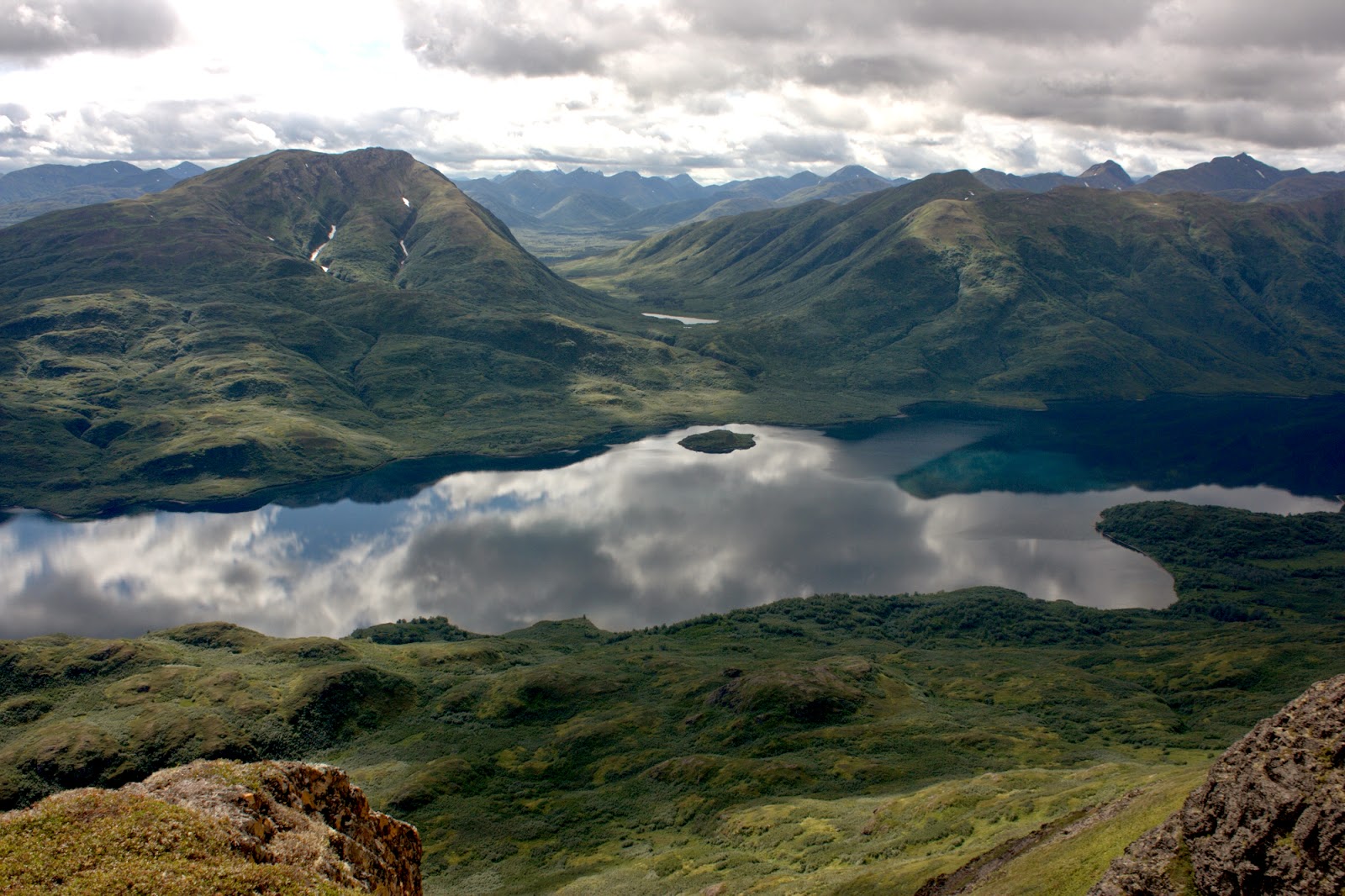
Little Togiak Lake, Wood-Tikchik State Park, Alaska.

The Alaska Salmon Program at the University of Washington has been doing research in the Bristol Bay region since 1946, well before Alaska became a state. One major focus of our work has been understanding the ecological effects of habitat diversity on Alaskan salmon stocks, now one of the world’s best examples of a productive and sustainable fishery. Hilborn et al. 2003 showed that the Bristol Bay sockeye salmon (Oncorhynchus nerka) are relatively stable in abundance and resilient to shifts in climate conditions because they are not one gigantic, panmictic population, but instead a metapopulation of independent breeding aggregations adapted to unique spawning habitat types (streams, rivers, and lake beaches). But how do these populations that are adapted to different habitats interact with each other on an evolutionary time scale? Are they on the road to speciation or does gene flow limit their divergence and possibly their adaptation to local conditions?

Despite the famous ability of pacific salmon to home to their natal spawning grounds after years in the ocean, dispersal rates among nearby populations have been measured to be 2–10%, potentially high enough to swamp the effects of ecologically divergent selection. However, even in the presence of considerable dispersal, gene flow may be limited if dispersers have low reproductive success in already-occupied habitats. Where local adaptation has arisen, dispersers between populations occupying distinct habitat types might be maladapted to their new habitat compared to philopatric (non-dispersing) individuals and dispersers between similar habitats, reducing gene flow and reinforcing local adaptation.

We set out to empirically assess the effect of local adaptation on the reproductive success of dispersers between beach- and stream-adapted populations. Beach-spawning fish, especially males, tend to be large and deep-bodied, while stream-spawning fish are more slender. Differences between these ecotypes have also been observed in other ecologically important traits such as egg size and migration timing. In order to isolate the fitness effects of local adaptation from those of dispersal itself, we compared the reproductive success of dispersers between populations that shared the same spawning habitat type with dispersers between ecologically distinct spawning habitat types.


Male and female sockeye salmon from the stream-spawning ecotype (above) and the beach-spawning ecotype (below). Photos: Tom Quinn.

To get direct measurements of individual dispersal and reproduction, we conducted exhaustive sampling of adults in two stream-spawning populations (A and C Creeks) every year from 2004 through 2010. We walked the full length of both streams every day during the spawning season (late July through late August), tagging any newly observed fish with unique IDs and noting the location of each previously tagged fish. We observed and fin-clipped a total of 4473 individuals in A Creek and C Creek in 2004 and 2005 (the parent years) and 2008, 2009, and 2010 (the years their offspring returned), plus 166 individuals that settled on the beach habitat in 2004 and 2005 (as a genetic baseline with which to identify dispersers from the beach to the streams). In the two parent years, 12% of sampled fish were immigrants (fish genetically assigned to a population other than the one in which they were sampled). C Creek had more immigrants from the other stream as well as from the beach than A Creek, but there was no clear sex bias in dispersing individuals. The number of individuals immigrating to the streams from the beach-spawning populations (N=108) was greater than the number of dispersers between stream-spawning populations (N=85).


Surveying C Creek. Photo: Jocelyn Lin.

Using pedigree reconstruction to calculate the number of returning adult offspring produced by each individual in the parental generation, we compared the lifetime reproductive success of all philopatric fish, dispersers between streams, and dispersers from adjacent lake beaches to the streams. We found that the reproductive success of dispersers between the two stream-adapted populations did not differ significantly from that of philopatric individuals, but immigrants from the beach population had significantly lower mean reproductive success than both philopatric fish and immigrants from the other stream. On average, beach-to-stream dispersers produced about one fewer offspring than between-stream dispersers, a reduction in fitness equivalent to almost half of the average reproductive success.

We don’t know the mechanistic reasons why dispersers from the beach produced fewer offspring. Morphological maladaptation to the stream environment could have limited the reproductive success of beach-adapted immigrants by reducing adult lifespan during the spawning period through selective bear predation or stranding in shallow water. Previous studies have shown that the abundant brown and black bears preferentially kill larger salmon (thereby selecting against them), but we found that dispersers from the beach were less likely to be found dead after being killed by bears and more likely to disappear without a trace. Recent PIT tagging work by Bentley et al. has shown that stream-spawning sockeye salmon show a wide variety of movement strategies, with many fish moving between stream and lake on a daily basis. It may be that the mere presence of bears indirectly affects the reproductive success of large-bodied dispersers by eliciting predator avoidance behavior and thereby limiting reproductive opportunity. Alternatively, reduced physical access to shallower areas of the stream could limit access to mates and spawning sites, encouraging the departure of larger individuals. Either way, adaptive behavioral differences between ecotypes may influence the conversion of dispersal into gene flow.


Spawning in the stream. Photo: Allan Hicks.

We usually expect that genetic differentiation, adaptive or otherwise, will only develop when diverging populations are insulated from gene flow by barriers to dispersal (either intrinsic or extrinsic). In our study, beach-to-stream dispersers were more prevalent than between-stream dispersers, suggesting that barriers to dispersal between habitat types are not strong in this system. The high fitness cost to dispersers that move between habitats might therefore be crucial to the maintenance of these morphologically and genetically recognizable stream- and beach-spawning ecotypes.

In the long term, we might expect that when dispersers have low reproductive success, selection will drive the evolution of intrinsic barriers to dispersal. However, additional factors might select against such barriers. For example, in dynamic metapopulations, rare subpopulation recolonization events might substantially bolster the long-term fitness of dispersal alleles even if dispersers have limited reproductive success in occupied subpopulations. Moreover, flexible behavior patterns in systems that allow for reversal of dispersal decisions could minimize the fitness cost of dispersal in unfavorable conditions. Thus, in many metapopulations, reduced immigrant reproductive success might be more important than barriers to dispersal for the maintenance of intraspecific biodiversity.

Reference:

Peterson DA, Hilborn R, & Hauser L (2014). Local adaptation limits lifetime reproductive success of dispersers in a wild salmon metapopulation. Nature Communications, 5.  DOI:10.1038/ncomms4696
http://www.nature.com/ncomms/2014/140417/ncomms4696/full/ncomms4696.html

Gordon Research Conference on Speciation: March 15–20, 2015

Hi everybody.  An upcoming conference on speciation has just been announced:

Gordon Research Conference on Speciation
Modes of Diversification, Ecological Mechanisms, and Genomic Signatures

March 15–20, 2015
Ventura, California, USA

A preliminary program is up with a great list of speakers.  More information is available at the conference’s home page.  Save the date!

Thursday, July 10, 2014

A small mammal with an outsized impact

[ This post is by Craig W. Benkman; I am just putting it up.  –B. ]

When we think of species having large and disproportionate impacts on communities, animals like sea otters come to mind. By eating and depleting sea urchins, sea otters prevent urchins from eating and depleting kelp. The huge difference between having kelp forests and their diverse community of fishes, sea lions, and eagles, versus largely kelp-less barrens arises simply from contemporary ecological processes; otters directly eating urchins and indirectly facilitating the increase in kelp. Such cascading effects are thought to be widespread both on land and in sea where you have strongly interacting species like mammals. Remove the mammals and the world is different. Unfortunately, we humans are very good at that.

Although less appreciated, strongly interacting predators and herbivores potentially have strong evolutionary effects on their prey. And, in the case in which the prey dominate a landscape, such evolutionary effects could be just as profound as those found for the more commonly studied trophic cascades of otters and their like. Our research indicates that Rocky Mountain lodgepole pine (Pinus contorta ssp. latifolia), which dominates tens of millions of hectares across the northern Rocky Mountains, is one such dominant species. The evolutionary effect is the result of differential seed predation by the aptly named pine squirrel (Tamiasciurus hudsonicus, also referred to as the American red squirrel; Talluto and Benkman 2014 Proceedings of the National Academy of Sciences USA 111:9543-9548; see also our 2013 paper in Ecology 94:1307-1316).


Map of lodgepole pine from Wikipedia. Rocky Mountain lodgepole pine occurs in and dominates much of the area highlighted by light green.

Driving across Yellowstone and other Rocky Mountain locales, one is struck by the variation in lodgepole pine seedling and sapling densities in areas recovering from fire. This variation has obvious consequences for the structure of plant communities varying from sparse pine seedlings and domination by various grasses and forbs to dense growth of pines with little else. Other components of the communities such as the various animal communities (e.g., birds, mammals, and invertebrate pollinators) must also vary accordingly.


A dense carpet of lodgepole pine saplings several years after a fire. (Photo from Wikipedia)

The key question is what causes the variation in the initial pine seedling density following fire. Ecosystem and landscape ecologists Monica Turner, Dan Tinker, and their colleagues found that the best predictor of seedling density after the 1988 Yellowstone fires was the frequency of serotiny in the pre-fire forest (Turner et al. 2003, Frontiers in Ecology and the Environment 1:351-358). Serotiny occurs when woody plants in fire-prone habitat encase their seeds for multiple years in woody structures (hard woody cones in lodgepole pine) creating an arboreal seed bank that is released soon after a stand-replacing fire. When the frequency of serotiny among the pines is high, large numbers of seeds are released from serotinous cones after fire sweeps through, resulting in large numbers of seedlings. Lower frequencies of serotiny result in fewer seeds available after the fire and many fewer seedlings. Turner, Tinker and colleagues found that the density of seedlings per hectare ranged from 600 when less than one percent of the trees were serotinous to 211,000 when 65% of the trees were serotinous. These remarkable differences resulted in dramatic differences in nutrient flows and how the communities developed after a fire.


Serotinous lodgepole pine cones remain closed with seeds secured inside for years until the heat from a fire causes the scales to open and shed their seeds. These cones are over 5 years old. (C. Benkman photo)

Non-serotinous cones open and seeds are shed several weeks after the seeds mature in early autumn. (C. Benkman photo)

Traditionally, forest ecologists have focused on variation in the frequency of fire to account for variation in the occurrence of serotiny. More frequent fires favor higher frequencies of serotiny, and observations, including those contrasting low and high elevations in Yellowstone, support such a relationship. However, the variation in serotiny mentioned above occurs in the lower-elevation lodgepole pine forests of Yellowstone where fire frequency is rather high and where one might expect the frequency of serotiny to be uniformly high if fire alone was the main selective agent driving the occurrence of serotiny.

This is where pine squirrels come in. Theoretically, a seed predator could select against serotiny by preferentially preying on seeds in the serotinous cones and thereby depleting the arboreal seed bank. Pine squirrels are such a predator. Both females and males defend separate territories year-round where they harvest, cache, and defend thousands of closed cones with seeds secured within. Because serotinous cones remain closed and hold their seeds for years if not decades, seeds in serotinous cones remain vulnerable to squirrels for years. In contrast, squirrels harvest non-serotinous cones almost exclusively during the several weeks between seed maturation and scale opening and seed shedding in autumn. Consequently, the overall probability of a squirrel harvesting a given serotinous cone is about 100 times higher than that for a non-serotinous cone. Depending on the density of squirrels, this can result in extremely strong selection against serotiny. Indeed, our models taking into account the life histories of the pines, differential seed predation, and fire frequency show that when squirrel densities exceed one and a half squirrels per hectare, selection by squirrels against serotiny overwhelms countering selection by fire favoring serotiny. At lower squirrel densities the balance between selection by squirrels and fire should set the frequency of serotiny.


Pine squirrel biting off the overlapping scales of a lodgepole pine cone to reach the underlying seeds. (C. Benkman photo)

Our model accounts quite well for the patterns of variation in the frequency of serotiny across Yellowstone and elsewhere. Both at both low elevations where fire frequency is high and at high elevations where fire frequency is lower, the frequency of serotiny is inversely related to the density of squirrels; as predicted by the models and observed, the average frequency of serotiny is higher at lower elevations where fire frequencies are higher. Our model also explains why the frequency of serotiny in ranges east and west of the Rockies, where squirrels were unable to colonize, is uniformly around 90 percent and exceeds the frequency found in areas with squirrels. Indeed, following a fire in the Cypress Hills, where there were no squirrels and the frequency of serotiny averages 92 percent, the density of seedlings was 2,500,000 per hectare!

Much of the variation in the frequency of serotiny, therefore, represents the outcome of two conflicting selection agents, one abiotic, fire, and one biotic, differential seed predation by pine squirrels. Importantly, at high enough squirrel densities the selection they exert overwhelms selection from even high frequencies of fire favoring serotiny. The balance of these conflicting selective agents in turn influences the density of seedlings after a fire with huge community and ecosystem consequences. Because serotiny is a genetically based trait with 11 “loci” accounting for over 50 percent of the variation in the trait (Parchman et al. 2012 Molecular Ecology 21:2991-3005), we can begin to link “genes” to ecosystems over vast expanses of the Rocky Mountains where lodgepole pine dominates the landscape, all mediated by the two main conflicting selection agents. In short, a small squirrel has an evolutionary impact with outsized ecological consequences.

Monday, July 7, 2014

Sometimes it’s better to be lucky than good

[ This post is by Devon Pearse; I am just putting it up. –B. ]

Identifying the genomic basis of complex, ecologically important phenotypes has become a major obsession among many evolutionary geneticists. Recently, some of the best successes in finding them have been in systems in which strong divergent selection has driven genetic changes at a few significant loci. These situations in the wild are analogous to the strong artificial selection imposed in plant and animal breeding. Certain traits selected for during the domestication process in dogs, for example, are determined by just a few genes of major effect rather than having the more polygenic architecture previously assumed. Similarly, examples of complex phenotypes with simple genetic architectures have been found in studies of wild organisms undergoing recent strong selection, such as those driven by anthropogenic impacts.

One such trait is smoltification, the process through which anadromous fishes mature from their freshwater juvenile rearing habitats into an ocean-going phase to grow to adulthood. This transformation is the epitome of a complex phenotype, involving changes in physiological, morphological, and behavioral traits preceding downstream migration to the ocean. And in some species, including the enigmatic salmonid species Oncorhynchus mykiss, undergoing this transformation is optional—individuals that smolt become ocean-going steelhead, while other individuals remain in freshwater to mature as rainbow trout. Not surprisingly, efforts to use genomic techniques such as GWAS and QTL mapping have identified numerous significant associations, but different studies have produced highly variable results, often identifying completely different chromosomal regions as important in determining individual expression of anadromy.


Photo: Anadromous and resident O. mykiss. Credit: Morgan Bond. 

This brings us to the subject of this post, recent studies in which my colleagues and I took a different approach (Martinez et al. 2011; Pearse et al. 2014). Taking advantage of pairs of wild populations above and below barriers to migration, we reasoned that, from the perspective of the above-barrier populations, selection would be extremely strong to stay above the falls—fish that migrate downstream can’t come back, so any gene that increases the probability of smoltification would rapidly remove itself from the above-barrier populations, never to return. Using a simple Fst-outlier approach, we detected parallel adaptive changes in the allele frequencies at multiple loci in multiple populations, many of which had been isolated above-barrier for just a few decades following introduction or dam construction. These patterns demonstrated that a large genomic region on chromosome Omy5 plays a key role in the evolution and expression of smoltification in nature, and that repeated evolution of the resident freshwater phenotype above-barriers has resulted in a parallel evolutionary genetic response in this region.


Allele frequencies of 55 SNP loci located on Omy5 in populations above and below barriers to migration. Orange and blue indicate frequencies of alleles associated with resident and anadromous populations, respectively. Loci are ordered left to right based on the strength of linkage disequilibrium between them. (from Pearse et al. 2014).

Given the hard selection in these above-barrier populations against alleles associated with downstream migration, how strong of an effect is required to create these population differences? A simple simulation study illustrates this, and shows that given reasonable population parameters, a fitness differential as small as 5-10% could explain the observed patterns of parallel evolution. Thus, the population-level allele frequency changes we detected, even though they occurred over extremely rapid evolutionary timescales, could be the result of fairly small shifts in individual probability of smoltification.

Simulations using PopGen (v3.3, 2008) show that a small reduction in relative fitness for AA individuals (RR=1.0, AR=0.95, AA=0.9) can reduce the frequency of the A allele over ~30 generations, even with a small population size (N=100).

Regardless of the apparent strength of the association between the Omy5 region and life-history variation in O. mykiss, it is important to remember the fundamental truth of complex phenotypes—they are complex. To use the analogy of playing cards, the hand that is dealt may represent an individual’s genetic makeup, but how it is played has a huge influence on the outcome (phenotype). And, unlike card games, the genetic hand that each individual human, fish, or other organism is dealt is spread across tens of chromosomes, with potentially 100s or 1000s of genes and segregating genomic regions, so it is hardly surprising that such variable associations between phenotype and genotype have been described. Some cards may be more influential than others (an ace might greatly increase an individual’s probability of ‘winning’), while the influence of other cards may depend on the combination of cards dealt—a three of hearts could be very important in a hand with two other 3s or a run of hearts! Finally, evolution may link important genes together through chromosomal inversions or other mechanisms; skewing the odds like a set of aces that are always dealt together, these ‘supergenes’ may combine to exert much greater influence on the phenotype. The long-awaited publication of a genome sequence for O. mykiss (Berthelot et al. 2014, Nature Communications) will greatly facilitate further exploration into the genomic architecture that maintains the linkage block on Omy5.


Photo: Ben Alfred (Flickr)

Moving forward, the challenge is now to determine the extent to which variation in genes associated with phenotypes at the population level influence individual phenotypic expression in nature. Even for single, large-effect regions, such as the one on Omy5, phenotypic plasticity and ecological interactions will have a strong influence on trait expression, much like human genetic information that provides a ‘risk factor’ for an individual patient’s likelihood of developing a given disease. And, as in humans, there may be huge differences in genetic architecture among populations across the range of diverse species in nature. Understanding this variability will be critical to improving both our understanding of the evolutionary genetic basis of complex phenotypes and to efforts to conserve this variation.


References:

Martínez, A., Garza, J.C. & Pearse, D.E. 2011 A microsatellite genome screen identifies chromosomal regions under differential selection in steelhead and rainbow trout. Transactions of the American Fisheries Society 140, 829-842.

Pearse, D. E., Miller, M. R., Abadía-Cardoso, A., & Garza, J. C. 2014. Rapid parallel evolution of standing variation in a single, complex, genomic region is associated with life history in steelhead/rainbow trout. Proc. Roy. Soc. B. 281: 20140012. http://dx.doi.org/10.1098/rspb.2014.0012

(And a tip o’ the hat to Robin Waples for an insightful chat a few years back that greatly encouraged me to pursue this work)

Friday, July 4, 2014

Carnival of Evolution #73: World Cup Edition

The 73rd Carnival of Evolution has been hosted by Pleiotropy, in a tour de force “World Cup Edition” of the Carnival.  The good news: we were a top-seeded team, tied for second place, based on the all-around evolutionary excellence of our nominated post, Katie Piechel’s “Add It Up: The Genetic Basis of Ecological Speciation”.  Go check out the Carnival to see how we did.

In honor of the World Cup, we have two additional items for your delectation:

The evolution of World Cup soccer balls through time.  Interesting, no?  I didn't realize the truncated icosahedron shape was such a modern thing.  Photo credit: Jens Heilmann.

And this is, of course, from Jerry Coyne’s website; I hope he doesn’t mind us propagating this meme, for it is a high-fitness meme indeed.

Predicting Speciation?

(posted by Andrew on behalf of Marius Roesti) Another year is in full swing. What will 2024 hold for us? Nostradamus, the infamous French a...